In Depth: Parameter tuning for Gradient Boosting
In this post we will explore the most important parameters of Gradient Boosting and how they impact our model in term of overfitting and underfitting.
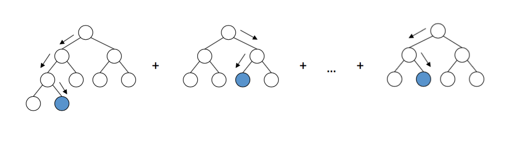
GB builds an additive model in a forward stage-wise fashion; it allows for the optimization of arbitrary differentiable loss functions. In each stage regression trees are fit on the negative gradient of the binomial or multinomial deviance loss function. Binary classification is a special case where only a single regression tree is induced.
We will use the Titanic Data from kaggle. For the sake of this post, we will perform as little feature engineering as possible as it is not the purpose of this post.
import numpy as np
import pandas as pd
import matplotlib as mpl
import matplotlib.pyplot as plt
Load train data
# get titanic & test csv files as a DataFrame
train = pd.read_csv("input/train.csv")
print train.shape
(891, 12)
train.head()
| PassengerId | Survived | Pclass | Name | Sex | Age | SibSp | Parch | Ticket | Fare | Cabin | Embarked | |
|---|---|---|---|---|---|---|---|---|---|---|---|---|
| 0 | 1 | 0 | 3 | Braund, Mr. Owen Harris | male | 22.0 | 1 | 0 | A/5 21171 | 7.2500 | NaN | S |
| 1 | 2 | 1 | 1 | Cumings, Mrs. John Bradley (Florence Briggs Th... | female | 38.0 | 1 | 0 | PC 17599 | 71.2833 | C85 | C |
| 2 | 3 | 1 | 3 | Heikkinen, Miss. Laina | female | 26.0 | 0 | 0 | STON/O2. 3101282 | 7.9250 | NaN | S |
| 3 | 4 | 1 | 1 | Futrelle, Mrs. Jacques Heath (Lily May Peel) | female | 35.0 | 1 | 0 | 113803 | 53.1000 | C123 | S |
| 4 | 5 | 0 | 3 | Allen, Mr. William Henry | male | 35.0 | 0 | 0 | 373450 | 8.0500 | NaN | S |
Check for missing values
#Checking for missing data
NAs = pd.concat([train.isnull().sum()], axis=1, keys=['Train'])
NAs[NAs.sum(axis=1) > 0]
| Train | |
|---|---|
| Age | 177 |
| Cabin | 687 |
| Embarked | 2 |
We will remove ‘Cabin’, ‘Name’ and ‘Ticket’ columns as they require some processing to extract useful features
# At this point we will drop the Cabin feature since it is missing a lot of the data
train.pop('Cabin')

# At this point names don't affect our model so we drop it
train.pop('Name')

# At this point we drop Ticket feature
train.pop('Ticket')

train.shape
(891, 9)
Fill the missing age values by the mean value
# Filling missing Age values with mean
train['Age'] = train['Age'].fillna(train['Age'].mean())
Fill the missing ‘Embarked’ values by the most frequent value
# Filling missing Embarked values with most common value
train['Embarked'] = train['Embarked'].fillna(train['Embarked'].mode()[0])
train.head()
| PassengerId | Survived | Pclass | Sex | Age | SibSp | Parch | Fare | Embarked | |
|---|---|---|---|---|---|---|---|---|---|
| 0 | 1 | 0 | 3 | male | 22.0 | 1 | 0 | 7.2500 | S |
| 1 | 2 | 1 | 1 | female | 38.0 | 1 | 0 | 71.2833 | C |
| 2 | 3 | 1 | 3 | female | 26.0 | 0 | 0 | 7.9250 | S |
| 3 | 4 | 1 | 1 | female | 35.0 | 1 | 0 | 53.1000 | S |
| 4 | 5 | 0 | 3 | male | 35.0 | 0 | 0 | 8.0500 | S |
‘Pclass’ is a categorical feature so we convert its values to strings
train['Pclass'] = train['Pclass'].apply(str)
Let’s perform a basic one hot encoding of categorical features
# Getting Dummies from all other categorical vars
for col in train.dtypes[train.dtypes == 'object'].index:
    for_dummy = train.pop(col)
    train = pd.concat([train, pd.get_dummies(for_dummy, prefix=col)], axis=1)
train.head()
| PassengerId | Survived | Age | SibSp | Parch | Fare | Pclass_1 | Pclass_2 | Pclass_3 | Sex_female | Sex_male | Embarked_C | Embarked_Q | Embarked_S | |
|---|---|---|---|---|---|---|---|---|---|---|---|---|---|---|
| 0 | 1 | 0 | 22.0 | 1 | 0 | 7.2500 | 0 | 0 | 1 | 0 | 1 | 0 | 0 | 1 |
| 1 | 2 | 1 | 38.0 | 1 | 0 | 71.2833 | 1 | 0 | 0 | 1 | 0 | 1 | 0 | 0 |
| 2 | 3 | 1 | 26.0 | 0 | 0 | 7.9250 | 0 | 0 | 1 | 1 | 0 | 0 | 0 | 1 |
| 3 | 4 | 1 | 35.0 | 1 | 0 | 53.1000 | 1 | 0 | 0 | 1 | 0 | 0 | 0 | 1 |
| 4 | 5 | 0 | 35.0 | 0 | 0 | 8.0500 | 0 | 0 | 1 | 0 | 1 | 0 | 0 | 1 |
labels = train.pop('Survived')
For testing, we choose to split our data to 75% train and 25% for test
from sklearn.model_selection import train_test_split

x_train, x_test, y_train, y_test = train_test_split(train, labels, test_size=0.25)
Let’s first fit a gradient boosting classifier with default parameters to get a baseline idea of the performance
from sklearn.ensemble import GradientBoostingClassifier

model = GradientBoostingClassifier()
model.fit(x_train, y_train)
GradientBoostingClassifier(criterion='friedman_mse', init=None,
              learning_rate=0.1, loss='deviance', max_depth=3,
              max_features=None, max_leaf_nodes=None,
              min_impurity_split=1e-07, min_samples_leaf=1,
              min_samples_split=2, min_weight_fraction_leaf=0.0,
              n_estimators=100, presort='auto', random_state=None,
              subsample=1.0, verbose=0, warm_start=False)
y_pred = model.predict(x_test)
We will AUC (Area Under Curve) as the evaluation metric. Our target value is binary so it’s a binary classification problem. AUC is a good way for evaluation for this type of problems
from sklearn.metrics import roc_curve, auc
false_positive_rate, true_positive_rate, thresholds = roc_curve(y_test, y_pred)
roc_auc = auc(false_positive_rate, true_positive_rate)
roc_auc
0.79286211093722836
learning_rate
learning rate shrinks the contribution of each tree by learning_rate.
learning_rates = [1, 0.5, 0.25, 0.1, 0.05, 0.01]
train_results = []
test_results = []
for eta in learning_rates:
    model = GradientBoostingClassifier(learning_rate=eta)
    model.fit(x_train, y_train)

    train_pred = model.predict(x_train)

    false_positive_rate, true_positive_rate, thresholds = roc_curve(y_train, train_pred)
    roc_auc = auc(false_positive_rate, true_positive_rate)
    train_results.append(roc_auc)

    y_pred = model.predict(x_test)


    false_positive_rate, true_positive_rate, thresholds = roc_curve(y_test, y_pred)
    roc_auc = auc(false_positive_rate, true_positive_rate)
    test_results.append(roc_auc)
from matplotlib.legend_handler import HandlerLine2D

line1, = plt.plot(learning_rates, train_results, 'b', label="Train AUC")
line2, = plt.plot(learning_rates, test_results, 'r', label="Test AUC")

plt.legend(handler_map={line1: HandlerLine2D(numpoints=2)})

plt.ylabel('AUC score')
plt.xlabel('learning rate')
plt.show()
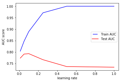
We see that using a high learning rate results in overfitting. For this data, a learning rate of 0.1 is optimal.
N_estimators
n_estimators represents the number of trees in the forest. Usually the higher the number of trees the better to learn the data. However, adding a lot of trees can slow down the training process considerably, therefore we do a parameter search to find the sweet spot.
n_estimators = [1, 2, 4, 8, 16, 32, 64, 100, 200]
train_results = []
test_results = []
for estimator in n_estimators:
    model = GradientBoostingClassifier(n_estimators=estimator)
    model.fit(x_train, y_train)

    train_pred = model.predict(x_train)

    false_positive_rate, true_positive_rate, thresholds = roc_curve(y_train, train_pred)
    roc_auc = auc(false_positive_rate, true_positive_rate)
    train_results.append(roc_auc)

    y_pred = model.predict(x_test)


    false_positive_rate, true_positive_rate, thresholds = roc_curve(y_test, y_pred)
    roc_auc = auc(false_positive_rate, true_positive_rate)
    test_results.append(roc_auc)
from matplotlib.legend_handler import HandlerLine2D

line1, = plt.plot(n_estimators, train_results, 'b', label="Train AUC")
line2, = plt.plot(n_estimators, test_results, 'r', label="Test AUC")

plt.legend(handler_map={line1: HandlerLine2D(numpoints=2)})

plt.ylabel('AUC score')
plt.xlabel('n_estimators')
plt.show()
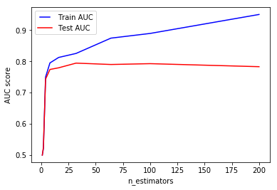
Increasing the number of estimators may result in overfitting also. In our case, using 32 trees is optimal.
max_depth
max_depth. This indicates how deep the built tree can be. The deeper the tree, the more splits it has and it captures more information about how the data. We fit a decision tree with depths ranging from 1 to 32 and plot the training and test errors.
max_depths = np.linspace(1, 32, 32, endpoint=True)
train_results = []
test_results = []
for max_depth in max_depths:
    model = GradientBoostingClassifier(max_depth=max_depth)
    model.fit(x_train, y_train)

    train_pred = model.predict(x_train)

    false_positive_rate, true_positive_rate, thresholds = roc_curve(y_train, train_pred)
    roc_auc = auc(false_positive_rate, true_positive_rate)
    train_results.append(roc_auc)

    y_pred = model.predict(x_test)


    false_positive_rate, true_positive_rate, thresholds = roc_curve(y_test, y_pred)
    roc_auc = auc(false_positive_rate, true_positive_rate)
    test_results.append(roc_auc)
from matplotlib.legend_handler import HandlerLine2D

line1, = plt.plot(max_depths, train_results, 'b', label="Train AUC")
line2, = plt.plot(max_depths, test_results, 'r', label="Test AUC")

plt.legend(handler_map={line1: HandlerLine2D(numpoints=2)})

plt.ylabel('AUC score')
plt.xlabel('Tree depth')
plt.show()
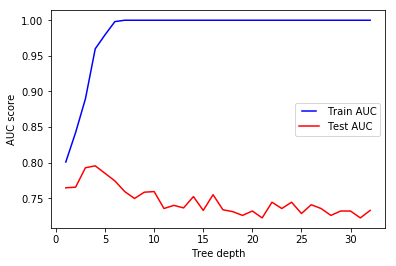
We see that our model overfits for large depth values. The tree perfectly predicts all of the train data, however, it fails to generalize the findings for new data
min_samples_split
min_samples_split represents the minimum number of samples required to split an internal node. This can vary between considering at least one sample at each node to considering all of the samples at each node. When we increase this parameter, the tree becomes more constrained as it has to consider more samples at each node. Here we will vary the parameter from 10% to 100% of the samples
min_samples_splits = np.linspace(0.1, 1.0, 10, endpoint=True)
train_results = []
test_results = []
for min_samples_split in min_samples_splits:
    model = GradientBoostingClassifier(min_samples_split=min_samples_split)
    model.fit(x_train, y_train)

    train_pred = model.predict(x_train)

    false_positive_rate, true_positive_rate, thresholds = roc_curve(y_train, train_pred)
    roc_auc = auc(false_positive_rate, true_positive_rate)
    train_results.append(roc_auc)

    y_pred = model.predict(x_test)


    false_positive_rate, true_positive_rate, thresholds = roc_curve(y_test, y_pred)
    roc_auc = auc(false_positive_rate, true_positive_rate)
    test_results.append(roc_auc)
from matplotlib.legend_handler import HandlerLine2D

line1, = plt.plot(min_samples_splits, train_results, 'b', label="Train AUC")
line2, = plt.plot(min_samples_splits, test_results, 'r', label="Test AUC")

plt.legend(handler_map={line1: HandlerLine2D(numpoints=2)})

plt.ylabel('AUC score')
plt.xlabel('min samples split')
plt.show()
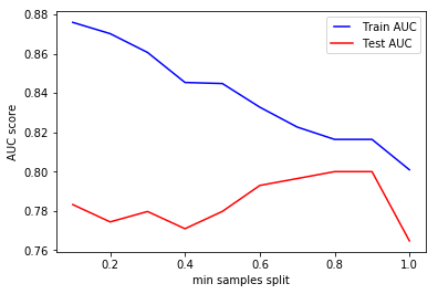
We can clearly see that when we require all of the samples at each node, the model cannot learn enough about the data. This is an underfitting case.
min_samples_leaf
min_samples_leaf is The minimum number of samples required to be at a leaf node. This similar to min_samples_splits, however, this describe the minimum number of samples of samples at the leafs.
min_samples_leafs = np.linspace(0.1, 0.5, 5, endpoint=True)
train_results = []
test_results = []
for min_samples_leaf in min_samples_leafs:
    model = GradientBoostingClassifier(min_samples_leaf=min_samples_leaf)
    model.fit(x_train, y_train)

    train_pred = model.predict(x_train)

    false_positive_rate, true_positive_rate, thresholds = roc_curve(y_train, train_pred)
    roc_auc = auc(false_positive_rate, true_positive_rate)
    train_results.append(roc_auc)

    y_pred = model.predict(x_test)


    false_positive_rate, true_positive_rate, thresholds = roc_curve(y_test, y_pred)
    roc_auc = auc(false_positive_rate, true_positive_rate)
    test_results.append(roc_auc)
from matplotlib.legend_handler import HandlerLine2D

line1, = plt.plot(min_samples_leafs, train_results, 'b', label="Train AUC")
line2, = plt.plot(min_samples_leafs, test_results, 'r', label="Test AUC")

plt.legend(handler_map={line1: HandlerLine2D(numpoints=2)})

plt.ylabel('AUC score')
plt.xlabel('min samples leaf')
plt.show()
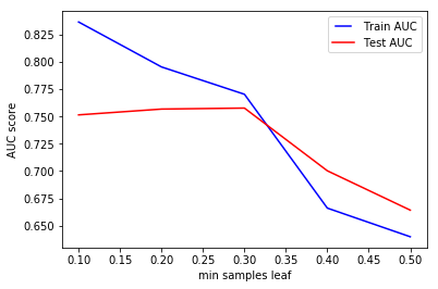
Same conclusion as to previous parameter. Increasing this value can cause underfitting.
max_features
max_features represents the number of features to consider when looking for the best split.
max_features = list(range(1,train.shape[1]))
train_results = []
test_results = []
for max_feature in max_features:
    model = GradientBoostingClassifier(max_features=max_feature)
    model.fit(x_train, y_train)

    train_pred = model.predict(x_train)

    false_positive_rate, true_positive_rate, thresholds = roc_curve(y_train, train_pred)
    roc_auc = auc(false_positive_rate, true_positive_rate)
    train_results.append(roc_auc)

    y_pred = model.predict(x_test)


    false_positive_rate, true_positive_rate, thresholds = roc_curve(y_test, y_pred)
    roc_auc = auc(false_positive_rate, true_positive_rate)
    test_results.append(roc_auc)
from matplotlib.legend_handler import HandlerLine2D

line1, = plt.plot(max_features, train_results, 'b', label="Train AUC")
line2, = plt.plot(max_features, test_results, 'r', label="Test AUC")

plt.legend(handler_map={line1: HandlerLine2D(numpoints=2)})

plt.ylabel('AUC score')
plt.xlabel('max features')
plt.show()
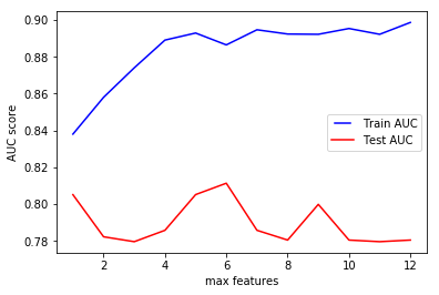
Increasing max_features to consider all of the features results in an overfitting in this case. Using max_features = 6 seems to get us the optimal performance.
You can also check other tree based models like Decision Tree and Random Forest