In Depth: Parameter tuning for SVC

In this post we will explore the most important parameters of Sklearn SVC classifier and how they impact our model in term of overfitting.

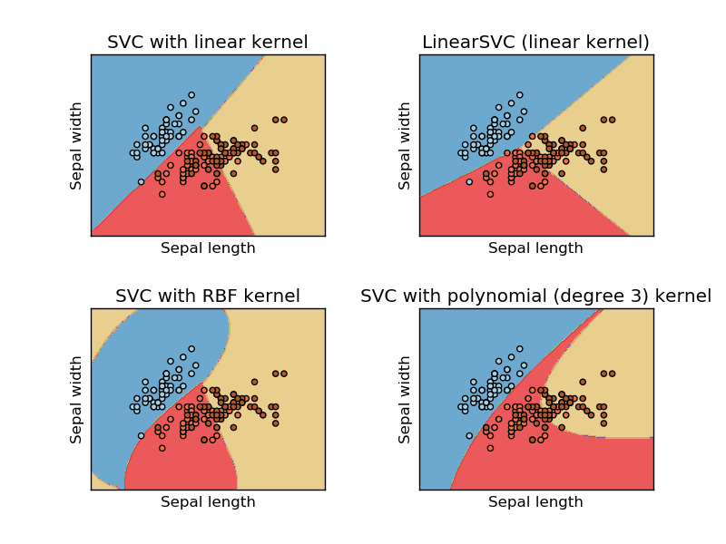
Support Vectors Classifier tries to find the best hyperplane to separate the different classes by maximizing the distance between sample points and the hyperplane.

We will use the Iris data from sklearn.

We start by loading the libraries and SVC

import numpy as np
import matplotlib.pyplot as plt
from sklearn import svm, datasets

%matplotlib inline

# import some data to play with
iris = datasets.load_iris()
X = iris.data[:, :2] # we only take the first two features. We could
 # avoid this ugly slicing by using a two-dim dataset
y = iris.target

We use the same plotting script for our plots.

def plotSVC(title):
    # create a mesh to plot in
    x_min, x_max = X[:, 0].min() - 1, X[:, 0].max() + 1
    y_min, y_max = X[:, 1].min() - 1, X[:, 1].max() + 1
    h = (x_max / x_min)/100
    xx, yy = np.meshgrid(np.arange(x_min, x_max, h),
 np.arange(y_min, y_max, h))

    plt.subplot(1, 1, 1)
    Z = svc.predict(np.c_[xx.ravel(), yy.ravel()])
    Z = Z.reshape(xx.shape)
    plt.contourf(xx, yy, Z, cmap=plt.cm.Paired, alpha=0.8)

    plt.scatter(X[:, 0], X[:, 1], c=y, cmap=plt.cm.Paired)
    plt.xlabel('Sepal length')
    plt.ylabel('Sepal width')
    plt.xlim(xx.min(), xx.max())
    plt.title(title)
    plt.show()

Kernel

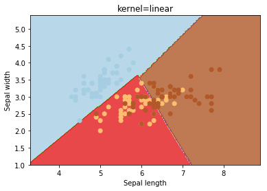
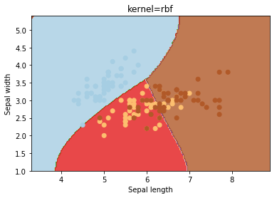
kernel parameters selects the type of hyperplane used to separate the data. Using ‘linear’ will use a linear hyperplane (a line in the case of 2D data). ‘rbf’ and ‘poly’ uses a non linear hyper-plane

kernels = ['linear', 'rbf', 'poly']

for kernel in kernels:
    svc = svm.SVC(kernel=kernel).fit(X, y)
    plotSVC('kernel=' + str(kernel))

gamma

gamma is a parameter for non linear hyperplanes. The higher the gamma value it tries to exactly fit the training data set

gammas = [0.1, 1, 10, 100]

for gamma in gammas:
    svc = svm.SVC(kernel='rbf', gamma=gamma).fit(X, y)
    plotSVC('gamma=' + str(gamma))

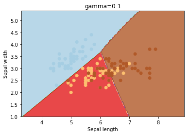
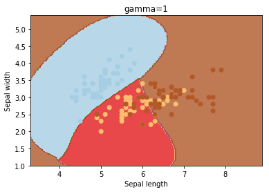
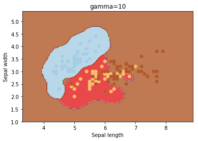
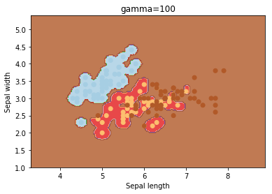
We can see that increasing gamma leads to overfitting as the classifier tries to perfectly fit the training data

C

C is the penalty parameter of the error term. It controls the trade off between smooth decision boundary and classifying the training points correctly.

cs = [0.1, 1, 10, 100, 1000]

for c in cs:
    svc = svm.SVC(kernel='rbf', C=c).fit(X, y)
    plotSVC('C=' + str(c))

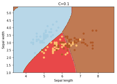
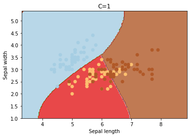
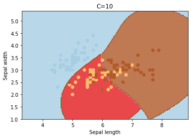
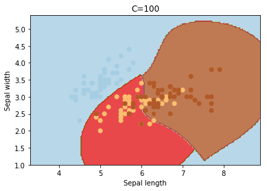
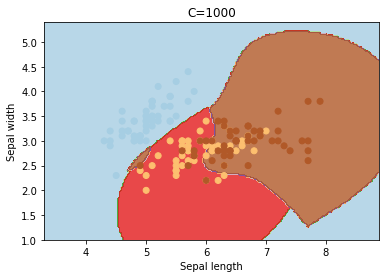
Increasing C values may lead to overfitting the training data.

degree

degree is a parameter used when kernel is set to ‘poly’. It’s basically the degree of the polynomial used to find the hyperplane to split the data.

degrees = [0, 1, 2, 3, 4, 5, 6]

for degree in degrees:
    svc = svm.SVC(kernel='poly', degree=degree).fit(X, y)
    plotSVC('degree=' + str(degree))

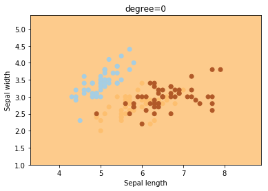
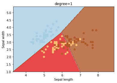
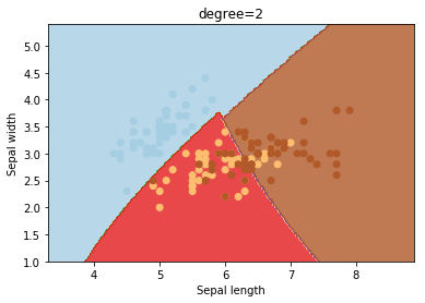
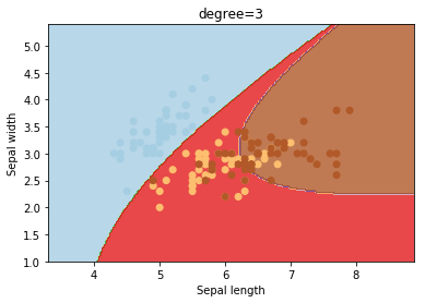
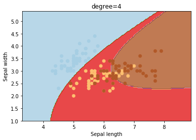
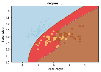
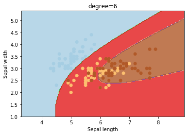
Using degree=1 is the same as using a ‘linear’ kernel. Also, increasing this parameters leads to higher training times.