Metflix: How to recommend movies - Part 1

In this series of posts, I will try to build a recommendation engine to recommend similar movies to a selected title or recommend movies to a user that rates a couple of movies. In Part 0, we downoaded the MovieLens dataset and created our user item sparse matrix. In this post, we go over some of the popular methods for recommendation, mainly:

• User Based Collaborative Filtering (UBCF)
• Item Based Collaborative Filtering (IBCF)
• Matrix Factorization (MF)

In the future posts, we will go over some of the evaluation metrics used to assess how good these models are, fine tune the selected model then deploy the model as a service and create a web service to interact with it, so stay tuned. Meanwhile let’s start with the first method.

User Based Collaborative Filtering

The general idea behind UBCF is that if two users agreed in their evaluation of an item in the past, they are likely to agree again in the future. This can be further generalized to a group of users instead of just a pair of users. As an example, if you ask your friends for some movie recommendations, you trust more the suggestions from friends that you share the same movie interests with than suggestions from friends with different interests.

In the example above, users rate different items (book, album, video, game) on a binary scale (like or dislike) and we want to know for a particular user if he likes or dislikes a certain video (That the user did not rate). To make a recommendation, we find the group of similar users and make a decision based on how they rated that item.

We compute the rating of a user u of an item i by the weighted sum of all other users’ ratings for item i as follow:

For the similarity function, there are two very common measures: Pearson-correlation and cosine similarity. Cosine similarity is basically the angle between the two users’ vectors.

For movie recommendations example, we select the top K most similar users based on the similarity matrix, aggregate their ratings, and then select the top N items as recommendations for our user.

Item Based Collaborative Filtering

Item Based Collaborative Filtering is exactly the same as the User Based but using item user interaction matrix. We obtain this matrix by transposing the user item matrix and then use the same similarity measures to get the similarity between items. We use the similarity score as weights to compute the rating for a particular (item, user) pair.

Item to Item Filtering

We can extend the Item Based Collaborative Filtering by recommending similar items to a target item. This is the basis for similar products recommendations shown on Amazon when you go to a product’s page. These recommendations are generated by computing a similarity matrix between all items and finding top K nearest items to a target item (nearest based on the similarity score).

Matrix Factorization

Matrix Factorization is usually applied in the context of dimensionality reduction: We try to reduce the dimension of our data while keeping as much information as possible. This can be achieved through Principal Component Analysis (PCA), Singular Value Decomposition (SVD) or Alternating Least Squares (ALS) which we will be using for this project.

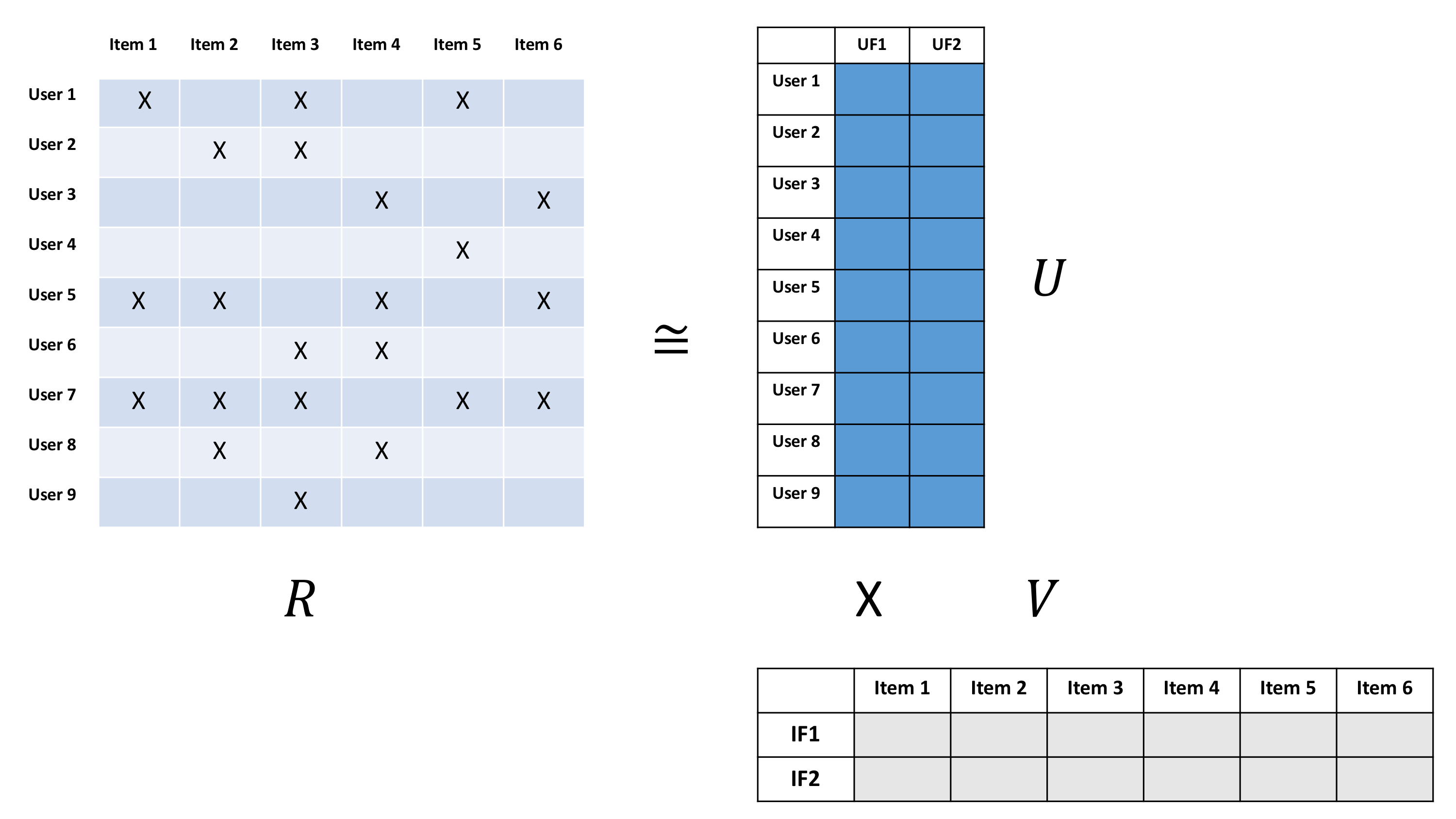
The main idea is to decompose the user item interaction matrix into a user matrix and item matrix of lower dimension than the original data.

If the user item matrix R is of dimension M x N, then we want to have a User matrix U and an item matrix V of dimensions M x K and K x N respectively with K < N. The two matrix U and V are called latent user features and latent item features. We don’t want the product of U and V to be exactly equal to R but we want to minimize the difference error and also apply some regularization to make sure we don’t overfit on the training data. Let’s express all of this in some equations:

We want to estimate the ratings matrix R as close as possible with a user matrix X and an item matrix Y:

And we want to minimize the difference between the real and the estimate rating matrices plus additional regularization terms for X and Y

To minimize our loss function we ALS. The basic idea is that at each iteration we fix one of the vectors as a constant and optimize for the other one and then do the opposite. That’s where the name Alternating Least Squares comes from.

When we fix Y and optimize X by taking the derivative at 0 for the loss function we get

Then we fix X with the optimized value from the previous step, and optimize Y by taking the derivative at 0 for the loss function we get

After running the algorithm for few iterations, we reach convergence. This algorithm has 3 parameters to tune: the number of latent factors to keep, the number of iterations to run the ALS for and the regularization term. These need to be optimized based on the data.

We will stop here for this post. In the next post, we will implement ALS for our data, get some recommendations and think of an evaluation metric to optimize our parameters for.